2. Accelerated Motion

Overview

Accelerated motion describes when an object's velocity is changing. In this unit, we will consider cases with constant acceleration.

Slides

Skills and Understanding

Understand that acceleration is the rate of change of velocity and know how it affects the motion of an object.
Analyze graphs of position, velocity, and acceleration.
Apply kinematic equations to solve problems including freefall.

Equations

\[ \begin{array}{cc} v = \frac{\Delta x}{\Delta t} \quad \quad \quad \quad & v_{f} = v_{i} + a \cdot \Delta t \\ a = \frac{\Delta v}{\Delta t} \quad \quad \quad \quad & \Delta x = \frac{1}{2} \left( v_{i} + v_{f} \right) \Delta t \\ v_{avg} = \frac{v_{i}+v_{f}}{2} \quad \quad \quad \quad & \Delta x = v_{i} \Delta t + \frac{1}{2} a \Delta t ^{2} \\ \quad \quad \quad \quad & v_{f}^{2} = v_{i}^{2} + 2 a \Delta x \end{array} \]

Vocabulary

Acceleration \(a\) is the rate at which velocity changes. It is calculated as \(a = \frac{\Delta v}{\Delta t}\)
Displacement is the change in position from the start to the end of a path. Given an initial position \(x_{i}\) and final position \(x_{f}\), the displacement \(\Delta x\) is calculated as \(\Delta x = x_{f} - x_{i}\)
Freefall describes when an object is falling due to gravity alone.
Velocity is the rate at which position is changing. It is calculated as \(v = \frac{\Delta x}{\Delta t}\)

2.1 Acceleration

Acceleration is change in velocity per time, \[ a = \frac{\Delta v}{ \Delta t} = \frac{v_{f} - v_{i}}{\Delta t} \ \]

A ball is thrown at 31 m/s. The ball hits a wall and bounces directly back, 24 m/s in the opposite direction. If the ball was in contact with the wall for 0.035 s, what was the acceleration during the bounce?

↓

Considering the ball starting in the positive direction, the ball is initially moving with velocity \[ v_{i} = 31 \text{ m/s} \] After the ball bounces off the wall, its velocity is \[ v_{f} = -24 \text{ m/s} \] We also have that \[ \Delta t = 0.035 \text{ s} \] Using the formula \[ a = \frac{v_{f} - v_{i}}{\Delta t} \] we can plug in to get \[ a = \frac{-24 - 31}{0.035} = -1571 \text{ m/s}^{2} \]

2.2 Position versus Time Graphs and Acceleration

When velocity was constant (acceleration was zero), position versus time graphs were linear. That was inline with our understanding that velocity was the slope of the position versus time graph, and constant slope results in a straight line. Now that we are considering acceleration, velocity is changing, so our position versus time graphs will no longer be linear.

Given the four samples of motion below, consider these questions:

Is the velocity positive or negative?
Is the acceleration positive or negative?
Is the person speeding up, or slowing down?
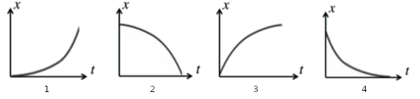
What would the graph of position versus time look tike?

Match each of the motion samples above to one of these position versus time graphs:

2.3 Velocity versus Time Graphs

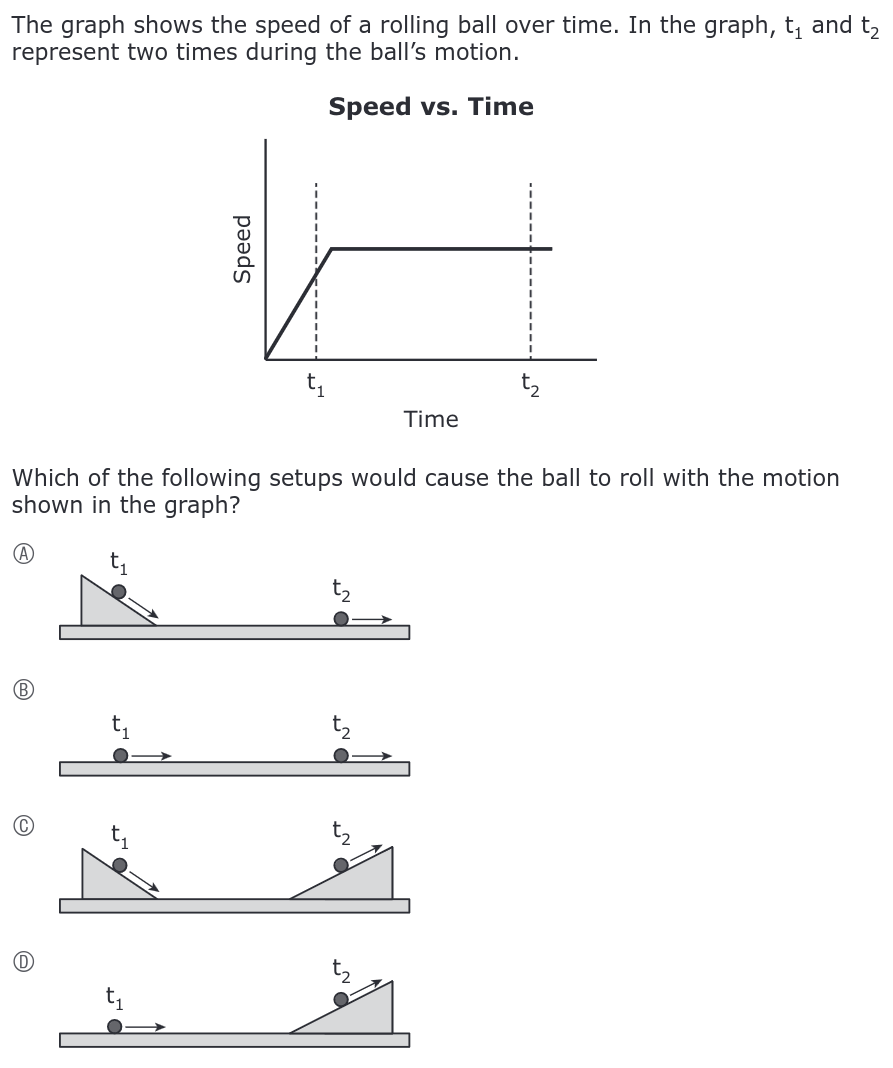
Source: 2022 MCAS

↓

The speed-versus-time graph represents an object that is speeding up at time \(t_{1}\) and maintaining a constant speed at \(t_{2}\). Scenario A matches the graph.

Source: 2022 MCAS

↓

In a velocity-versus-time graph, the area "under" the curve is equal to the displacement. Over the time interval from 4 to 8 s, the displacement is \[4 \cdot 30 = 120 \text{ m}\]

2.4 Kinematic Equations

Assuming constant acceleration, there are four common equations: \[ v_{f} = v_{i} + a \cdot \Delta t \] \[ \Delta x = \frac{1}{2} \left( v_{i} + v_{f} \right) \Delta t \] \[ \Delta x = v_{i} \Delta t + \frac{1}{2} a \Delta t ^{2} \] \[ v_{f}^{2} = v_{i}^{2} + 2 a \Delta x \] Each of these equations is useful in a different way. Note that the first equation has no \(\Delta x\), the second has no acceleration \(a\), the third requires no \(v_{f}\), and the last has no \(\Delta t\).

When presented with a kinematic physics problem, identifying the Givens and the Unknown helps us to choose the appropriate Equation to use.

A car is traveling at \(21\) m/s when it begins to accelerate at a rate of \(4.5\) m/s\(^{2}\) for 3.1 s. How far does the car travel during those 3.1 s?

↓

We are Given that \[ v_{i} = 21 \text{ m/s} \] \[ a = 4.5 \text{ m/s}^{2} \] \[ \Delta t = 3.1 \text{ s} \] and we want to find the Unknown \(\Delta x\). The Equation \[ \Delta x = v_{i} \Delta t + \frac{1}{2} a \Delta t ^{2} \] has everything we are given as well as what we are trying to find. Plugging in we have \[ \Delta x = (21) (3.1) + \frac{1}{2} (4.5) (3.1)^{2} = 87 \text{ m} \]

2.5 Freefall

Freefall describes when an object is accelerating due only to gravity. The acceleration due to gravity at the surface of Earth is approximately -9.81 m/s\(^{2}\), but we'll often use the value \(-10\) m/s\(^{2}\).

A tennis ball is dropped from rest at a height of 3.8 m. How much time will it take for the ball to hit the ground?

↓

We are given \[\Delta y = -3.8 \text{ m}\] \[a = -10 \text{m/s}^{2} \] \[v_{i} = 0 \text{ m/s} \] and we are looking for \(\Delta t\). We can use the formula \[ \Delta y = v_{i} \Delta t + \frac{1}{2}a \Delta t^{2} \] Plugging into this formula we have \[ -3.8 = (0)\Delta t + \frac{1}{2} (-10) \Delta t^{2} \] which we can solve to get \[ \Delta t = \sqrt{ \frac{2 \cdot (-3.8)}{-10}} \approx 0.87 \text{ s}\]