Collaborative Data Science

This page contains resources for a session at the 2023 NCTM Virtual Conference.

Slides:

Introduction

A classifier is an algorithm which takes some input and categorizes that input based on features (recognizable patterns). There are several popular algorithms for automating the identification of features in data. Some examples of classification problems include:

• Distinguishing spam from non-spam in email.
• Object recognition in images.
• Speech recognition in audio.
• Likely winners in sporting events.

The activity presented here is a manual feature engineering project, classifying handwritten digits from the famous MNIST dataset. Given examples of handwritten digits, we ask: what features can we identify or create which are effective at distinguishing digits from one another? The project is iterated with increasingly difficult tasks:

1. Distinguish between 0s and 1s.
2. Determine one digit that you can distinguish from the nine others.
3. Distinguish more digits!
4. Improve performance.
5. Try it again with a new model.

Some of the reasons I like this project are:

• Concepts utilized in this type of problem are a fundamental in data-based applied mathematics.
• The collaboration is natural in a project of this type, so it doesn't feel added on.
• The project facilitates frequent translating between intuition and formalization, between abstract and algorithmic thinking.
• It has low floors, high ceilings, and wide walls. Every student can contribute, there is no limit on how complex solutions may become, and every student could find different succesful solutions.

You can find some code and links to Python Notebooks below, but think of those as bonus features if you are interested. They aren't necessary to complete the main project.

Get to know the data

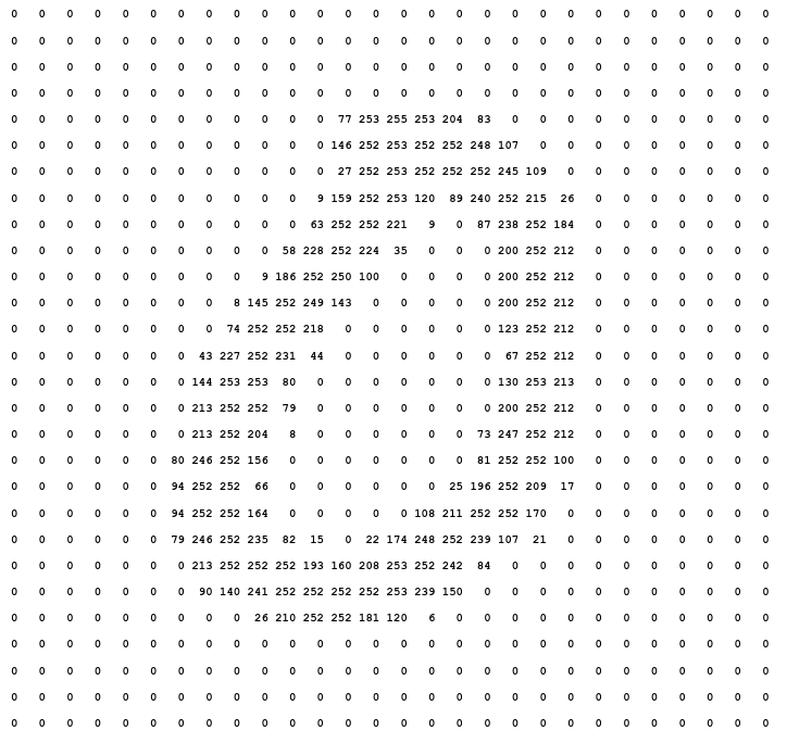
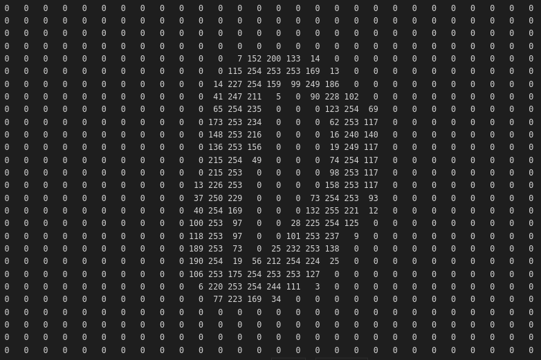
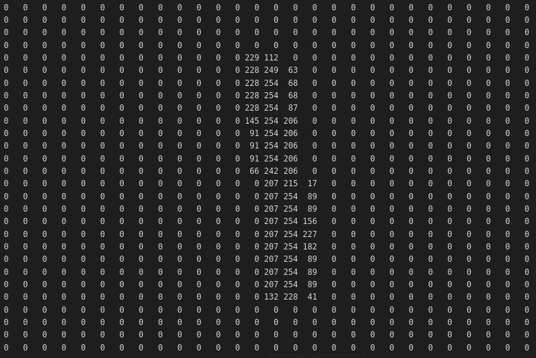
A brief history of MNIST can be viewed at https://www.youtube.com/watch?v=oKzNUGz21JM. An archive of the images saved as PNGs is available from https://github.com/myleott/mnist_png. Each image is \(28 \times 28\) pixels of grayscale values. Here is an \(8\):

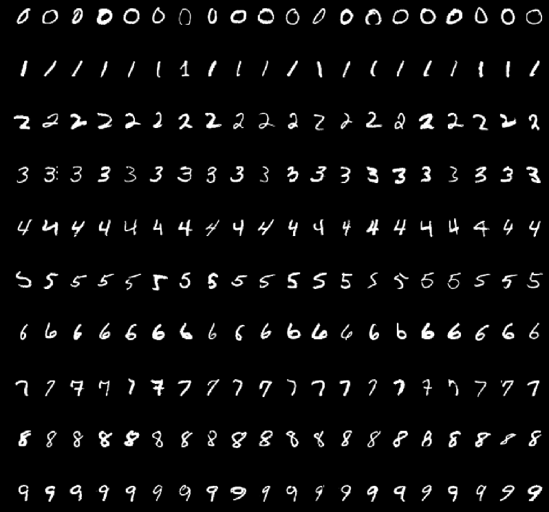
Visualizing some more of the digits, we can get a sense of dataset:

If you have some coding experience, then you can do a lot with this dataset. But you can also do a lot with a simple spreadsheet! Take a look at this sheet. Each row in the spreadsheet represents a single image. The first column is the label of what digit is in the image. The next 784 columns are the 784 pixel values in a single image.

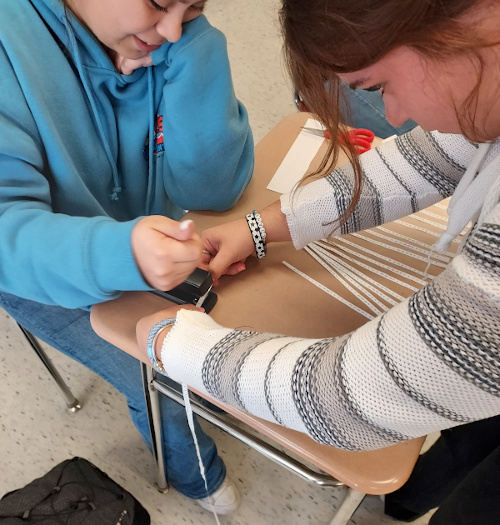
It can be confusing, thinking of a 2D image as 1D list of numbers. An activity that can be helpful for starting to think about image data in this way is to physically cut out the rows of a digit's pixel values and create a physical representation of an image vector.

Below are some images of students cutting up their digits and either stapling or taping all 28 rows of image data together into a single image vector. The result is a effectively a physical version of our spreadsheet!

Feature Engineering

Now that we are familiar with our data, let's explore deeper and uncover some features that might help us to distinguish between \(0\)s and \(1\)s in our first spreadsheet. What features do \(0\)s have that \(1\)s don't, or the other way around?

While we will be working with the data in the spreadsheet, perhaps thinking back to the 2D images will inspire some ideas for distinguishing features.

The above images are only single samples, but what do you notice and wonder? Below are samples of student responses, hidden to avoid spoilers.

Click for student responses

• The \(0\)s will be wider.
• The left-most part of the \(1\) is only a few pixels apart from the right-most part.
• The \(0\) has more non-zero pixels.
• You can add up all of the pixel values, and \(0\)s will have a higher number.
• I wonder how many \(1\)s have the base and the hat.
• If you go across the middle of the \(0\) (horizontally), it goes zeros, numbers, zeros, numbers, zeros. With \(1\)s, it just goes zeros, numbers, zeros.
• If you got straight down the middle, the \(1\) has a lot more non-zero pixels.
• I wonder if all of the \(1\)s are centered in the image.
• I wonder if some \(1\)s are slanted.
• If the middle pixel is zero, it is a \(0\). If it is not, then it is a \(1\)

Some features will be relatively easy to calculate using a spreadsheet formula. Other features, while feasible, are more abstract and challenging to capture algorithmically. Some features will be effective for classification, while others will be less robust.

Example Feature

Let's try one of the simpler features: sum all of the pixel values in each image. Our hope is that we will be able to distinguish \(0\)s because their sums will be higher than those of \(1\)s.

Each feature we create will be in the form of a spreadsheet formula, and we'll keep them in the far right columns. In the far right column of our 0 and 1 spreadsheet, we will enter two formulas. In ADF2, we enter:

=A2

This makes a copy of the digit label for our convenience. Then in ADG2, we enter:

=sum(B2:ADE2)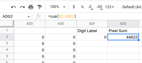

This formula sums all of the 784 pixel values.

We can select both of our new formula cells and double-click the blue square to auto-fill the columns. We have a feature!

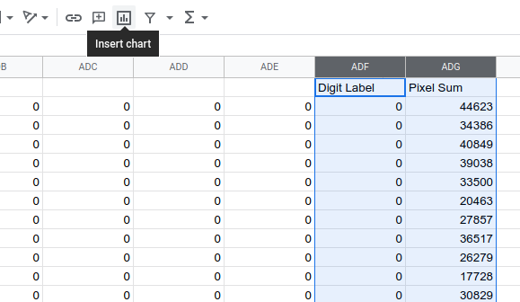
Let's make a scatter plot of columns ADF and ADG to get a sense of how distinguishing this feature is:

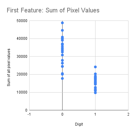
Not too shabby!

Classifier

So we have a feature that looks like it can nearly distinguish \(0\)s from \(1\)s. Let's utilize that feature to make a classifier. In ADH2, let's define a formula to classify the image as \(0\) or \(1\):

=if(ADG2>20000,0,1)

This formula looks at the value immediately to the left and if it is greater than \(20000\), it predicts \(0\), otherwise it predicts \(1\). Based on our scatter plot, this roughly seems reasonable.

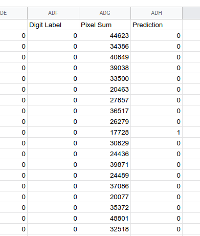
It works! Well, at least with our training data it classifies correctly on 37 out of 40 images. You can get 40/40 either by finding a great feature, or combining more than one feature.

Conclusions

We can identify data features and use them to create classifiers. Go forth, find new features, and maybe even combine them to improve accuracy.

It is important when working on data projects like this one to reflect.

• Our classifier is built (trained) on a partiuclar dataset
• The data captures particular cultural conventions
• Our biases are baked into our classifier via the decisions we made along the way
• Our classifier is a predictor, not a judge

To clarify that last point. Our classifier is a feature-based model for making a prediction based on numerical nearness to stereotypes. Given some input data, it characterizes the 1-ness or the 0-ness of that data as defined by the conventions in the data and the decisions we made about what features to include.

Data projects are awesome and they are a fantastic window through which we might observe and reflect on the consequences of applied mathematics.